Module 5: Theory of Computation

Module 5: Overview

Theory of Computation (ToC) is the branch of computer science that asks the most fundamental questions about computing itself: What problems can be solved by a computer at all? What problems can be solved efficiently? And what formal models underlie every computation we perform? ToC provides the mathematical foundations that every other area of CS rests on.

The field is traditionally divided into three pillars, each building on the last. This module follows that progression.

I Automata Theory
1Section 1: Finite Automata — DFA and NFA
2Section 2: Regular Languages and Expressions
3Section 3: Context-Free Languages and Pushdown Automata
II Computability Theory
4Section 4: Turing Machines
5Section 5: Decidability and the Halting Problem
III Complexity Theory
6Section 6: P, NP, and NP-Completeness

Notation Reference

The following symbols appear throughout this module. Refer back here as needed.

Σ: The alphabet — a finite, non-empty set of symbols (e.g. {0, 1})
Σ*: The set of all strings over Σ, including the empty string ε
ε: The empty string — a string of length zero
w: A generic string (word) over Σ
|w|: The length of string w
L: A language — any subset of Σ*
Q: A finite set of states
q₀: The start state (initial state)
F: The set of accept states (final states)
δ: The transition function
M: A generic machine (DFA, NFA, PDA, or TM)
L(M): The language recognised by machine M
⌶: A Turing Machine accepts (halts in accept state)
⊢: A configuration yields the next configuration in one step
P: Problems solvable in polynomial time
NP: Problems verifiable in polynomial time
≤ ᶹ: Polynomial-time many-one reduction

Section 1: Finite Automata — DFA and NFA

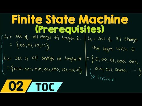
A finite automaton is the simplest model of computation. It reads an input string one symbol at a time, transitions between a finite set of states, and either accepts or rejects the string when it reaches the end. Despite their simplicity, finite automata model real systems — lexical analysers, network protocols, regular expression engines, and digital circuits.

1.1 Deterministic Finite Automata (DFA)

A DFA is a 5-tuple M = (Q, Σ, δ, q₀, F) where:

Formal definition

Q       — a finite set of states
Σ       — a finite alphabet
δ       — the transition function:  Q × Σ → Q
q₀      — the start state,           q₀ ∈ Q
F       — the set of accept states,  F ⊆ Q

M accepts string w = w₁w₂...wₙ if there exists a sequence of states
r₀, r₁, ..., rₙ such that:
  (1) r₀ = q₀                        (start in the start state)
  (2) δ(rᵢ, wᵢ₊₁) = rᵢ₊₁  for 0 ≤ i < n  (follow transitions)
  (3) rₙ ∈ F                         (end in an accept state)

A key property of DFAs is determinism: from every state, on every possible input symbol, there is exactly one transition. There is never any ambiguity about which state to move to next.

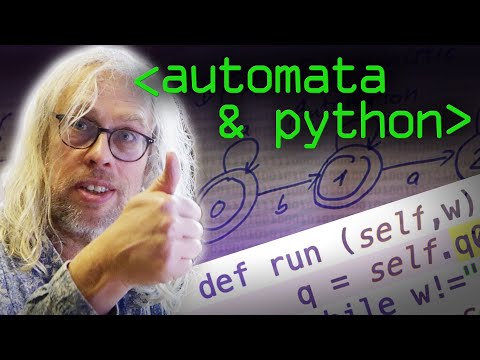
Example: The following DFA recognises the language L = { w ∈ {0,1}* | w ends in 1 } — all binary strings whose last symbol is 1. It has two states: q₀ (last symbol was 0, or no input yet) and q₁ (last symbol was 1). Only q₁ is an accept state.

State	On input 0	On input 1	Accept?
→ q₀	q₀	q₁	No
q₁	q₀	q₁	Yes

Tracing the string 1011: start in q₀ → read 1 → q₁ → read 0 → q₀ → read 1 → q₁ → read 1 → q₁. We end in q₁ (an accept state), so 1011 is accepted. ✓ Tracing 10: q₀ → q₁ → q₀ — end in q₀, rejected. ✗

1.2 Nondeterministic Finite Automata (NFA)

A NFA relaxes the determinism requirement. From a given state, on a given symbol, the transition function may produce zero, one, or many possible next states. NFAs also allow ε-transitions — transitions taken without consuming any input symbol.

NFA — 5-tuple

N = (Q, Σ, δ, q₀, F)

The only difference from a DFA:
  δ : Q × (Σ ∪ {ε}) → 𝒫(Q)   (power set of Q — a *set* of states, possibly empty)

An NFA accepts a string if at least one possible computation path leads to an accept state. You can think of the NFA as exploring all paths simultaneously (or "guessing" the right one). NFAs are often much easier to construct than equivalent DFAs.

Theorem — DFA/NFA Equivalence (Subset Construction)

Every NFA has an equivalent DFA that recognises exactly the same language. Given an NFA with n states, the equivalent DFA has at most 2ⁿ states (one for each subset of the NFA's state set). This is called the subset construction or powerset construction.

The subset construction works by making each state of the new DFA correspond to a set of NFA states. The DFA starts in the ε-closure of the NFA's start state, and transitions are computed by unioning the NFA transitions of every state in the current set, then taking the ε-closure of the result.

Property	DFA	NFA
Transitions per state/symbol	Exactly 1	0, 1, or many
ε-transitions	Not allowed	Allowed
Acceptance	Unique path ends in accept state	Any path ends in accept state
Expressive power	Exactly the regular languages	Exactly the regular languages
Ease of construction	Often complex	Often simpler to design

Useful Links

Cornell CS2800: DFAs GeeksForGeeks: Finite Automata ODU: NFA Definitions and Examples Wikipedia: Powerset Construction

Useful Videos

Watch on YouTube

Section 2: Regular Languages and Expressions

The class of languages recognised by DFAs is called the regular languages. Regular languages can also be described by regular expressions — a compact algebraic notation. Kleene's theorem establishes that these two characterisations describe exactly the same class of languages.

2.1 Regular Expressions

A regular expression (regex) over alphabet Σ is built from the following primitives and operations:

Regular expression syntax

Base cases:
  ε          matches the empty string
  a          matches the single symbol a ∈ Σ
  ∅          matches nothing (empty language)

Operations (R and S are regular expressions):
  R | S      union: matches strings in R or S
  R ⋅ S      concatenation: matches a string in R followed by one in S
  R*         Kleene star: matches zero or more concatenations of R
  (R)        grouping

Examples over Σ = {0, 1}:

Regex examples

(0 | 1)*           — all binary strings (including ε)
(0 | 1)* 1         — all binary strings ending in 1
0* 1 0*            — exactly one 1, any number of 0s
(01)*              — strings that are repetitions of "01": ε, 01, 0101, 010101, ...
0* (1 0* 1 0*)* 0* — strings with an even number of 1s

Theorem — Kleene's Theorem

A language L is regular if and only if it is described by a regular expression. More precisely: the class of languages recognised by DFAs = the class of languages recognised by NFAs = the class of languages described by regular expressions.

2.2 Closure Properties

The regular languages are closed under the following operations — meaning the result of applying them to regular languages is always also regular: union, concatenation, Kleene star, complementation, intersection, difference, and reversal. Closure properties are powerful tools for proving a language is regular or for constructing DFAs for complex languages by composing simpler ones.

2.3 The Pumping Lemma — Proving Non-Regularity

Not every language is regular. The Pumping Lemma gives us a tool to prove that a language is not regular by contradiction.

Theorem — Pumping Lemma for Regular Languages

If L is a regular language, then there exists a pumping length p ≥ 1 such that for every string w ∈ L with |w| ≥ p, we can write w = xyz where:

  (1) xyⁱz ∈ L for all i ≥ 0   (pumping condition)
  (2) |y| ≥ 1   (y is non-empty)
  (3) |xy| ≤ p   (the pump is near the start)

Example — proving L = {0ⁿ1ⁿ | n ≥ 0} is not regular:

Pumping Lemma proof sketch

Assume for contradiction that L is regular with pumping length p.
Choose w = 0ᷭ 1ᷭ  (p zeros followed by p ones).  |w| = 2p ≥ p.

By the Pumping Lemma, w = xyz where |xy| ≤ p and |y| ≥ 1.
Since |xy| ≤ p and w starts with p zeros,
  x and y consist entirely of 0s.
  Let y = 0ᵏ for some k ≥ 1.

Now pump: consider xy²z = x y y z.
  This string has p + k zeros but still p ones (y only added zeros).
  So xy²z = 0ᷯ₊ᵏ 1ᷭ  with k ≥ 1.
  But 0ᷯ₊ᵏ 1ᷭ ∉ L  because p + k ≠ p.

Contradiction! ∴ L is not regular.  ▮

Useful Links

Cornell CS2800: Kleene's Theorem GeeksForGeeks: Pumping Lemma Wikipedia: Regular Expressions (formal theory)

Useful Videos

Watch on YouTube

Section 3: Context-Free Languages and Pushdown Automata

Regular languages cannot describe all languages we care about in computer science. The language {0ⁿ1ⁿ} — which requires counting — is not regular, yet it is very naturally described by a grammar. Context-free languages (CFLs) are the next rung on the Chomsky hierarchy, characterised by context-free grammars (CFGs) and equivalent to pushdown automata (PDAs). Most programming language syntax is context-free.

3.1 Context-Free Grammars (CFGs)

We met CFGs briefly in Module 4 (Section 2) in the context of defining programming language syntax. Formally, a CFG is a 4-tuple G = (V, Σ, R, S):

Formal definition — CFG

V       — a finite set of variables (non-terminals)
Σ       — a finite set of terminals  (V ∩ Σ = ∅)
R       — a finite set of rules (productions): V → (V ∪ Σ)*
S       — the start variable,  S ∈ V

A string w ∈ Σ* is in L(G) if it can be derived from S by repeatedly replacing a variable with the right-hand side of one of its rules.

CFG — language {0ⁿ1ⁿ | n ≥ 0}

G = ({S}, {0, 1}, R, S)

Rules R:
  S → 0 S 1   (wrap the current string with one 0 and one 1)
  S → ε        (base case: the empty string)

Derivation of 000111:
  S ⇒ 0S1 ⇒ 00S11 ⇒ 000S111 ⇒ 000ε111 = 000111  ✓

3.2 Ambiguous Grammars

A grammar is ambiguous if some string has more than one distinct parse tree (or equivalently, more than one leftmost derivation). Ambiguity is a problem for programming languages because it means a source string could be interpreted in multiple ways. The classic example is the dangling-else problem in C-like languages — which if does an else belong to? Disambiguating grammars (or handling ambiguity via precedence rules) is a major concern of parser design.

3.3 Pushdown Automata (PDAs)

A pushdown automaton is an NFA augmented with an unbounded stack. At each step, the PDA reads an input symbol (or ε), pops the top of the stack, transitions to a new state, and pushes a string onto the stack. The stack provides the memory needed to handle languages like {0ⁿ1ⁿ} — push a symbol for each 0 read, pop for each 1.

Theorem — CFG/PDA Equivalence

A language is context-free if and only if it is recognised by a pushdown automaton. Every CFG can be converted to an equivalent PDA, and vice versa.

3.4 The Pumping Lemma for CFLs

Just as regular languages have a pumping lemma, so do context-free languages. The CFL version is more complex: sufficiently long strings can be split into five parts uvxyz where the middle portions v and y can be pumped simultaneously. The canonical non-CFL proven with this lemma is {aⁿbⁿcⁿ | n ≥ 0} — the stack can match two counts, but not three simultaneously.

Where CFLs appear in practice: The syntax of nearly every programming language is defined by a CFG and parsed by a pushdown automaton (via an LL or LR parser). However, some language features — such as checking that every variable is declared before use — are context-sensitive, not context-free, and require additional passes beyond parsing.

Useful Links

GeeksForGeeks: Context-Free Grammars University of Rochester: CFGs Wikipedia: Pushdown Automata Wikipedia: Pumping Lemma for CFLs

Useful Videos

Watch on YouTube

Section 4: Turing Machines

To study what computers can and cannot do, we need a model powerful enough to capture everything any real computer can compute. Alan Turing introduced the Turing Machine in 1936 — a simple abstract device that nevertheless matches the computational power of any physical computer ever built or conceivable.

4.1 Formal Definition

A Turing Machine is a 7-tuple M = (Q, Σ, Γ, δ, q₀, q_acc, q_rej):

Formal definition — Turing Machine

Q            — a finite set of states
Σ            — the input alphabet  (⊔ ∉ Σ, where ⊔ is the blank symbol)
Γ            — the tape alphabet   (Σ ∪ {⊔} ⊆ Γ)
δ            — the transition function:
                 Q\{qᵀᵃᵍ, qᵣᵉʸ} × Γ → Q × Γ × {L, R}
                 (state, tape symbol) → (new state, write symbol, move L or R)
q₀           — the start state
qᵀᵃᵍ         — the accept state  (halts and accepts)
qᵣᵉʸ         — the reject state  (halts and rejects, qᵣᵉʸ ≠ qᵀᵃᵍ)

The TM has an infinite tape divided into cells, each holding one symbol from Γ. A read/write head sits over one cell at a time. At each step, the machine reads the current cell, writes a symbol, moves left (L) or right (R), and transitions to a new state. The tape is initialised with the input string followed by blank symbols (⊔).

4.2 Example — Recognising {0ⁿ1ⁿ0ⁿ}

Here is an informal description of a TM that recognises { 0ⁿ1ⁿ0ⁿ | n ≥ 1 } — a language that is not context-free, demonstrating the power beyond PDAs:

TM — high-level description

Input: a string w over {0, 1}

1. Scan left to right. If the tape is blank, ACCEPT (empty string not in language here).
2. Mark the leftmost unmarked 0 (replace with X).
3. Scan right past 0s to the first 1. If none, REJECT.
   Mark it (replace with Y).
4. Scan right past 1s to the first 0 in the trailing group. If none, REJECT.
   Mark it (replace with Z).
5. Scan left to the beginning (past Xs, Ys, Zs).
6. Repeat steps 2-5 until all 0s in the first group are marked.
7. Scan the tape: if all 1s are marked (Y) and all trailing 0s are marked (Z),
   ACCEPT. Otherwise REJECT.

4.3 The Church-Turing Thesis

Church-Turing Thesis (informal)

Every effectively computable function — every function that can be computed by any algorithm, any physical computer, any conceivable mechanical process — can be computed by a Turing Machine.

This is a thesis, not a theorem — it cannot be formally proved because "effectively computable" is an informal notion. But it has been corroborated by every known model of computation: λ-calculus, recursive functions, register machines, RAM machines, and modern computer architectures all turn out to be equivalent in power to Turing Machines.

4.4 TM Variants

Many extensions of the basic TM have been studied. All are equivalent in computational power, which strengthens the Church-Turing thesis:

Variant	Description	Equal in power?
Multi-tape TM	Multiple tapes and heads operating in parallel	Yes
Nondeterministic TM	Transition function returns a set of possible next steps	Yes
Enumerator	Prints (enumerates) all strings of a language one by one	Yes
Random-access TM	Can access any tape cell in O(1) (like RAM)	Yes
Quantum TM	Uses quantum superposition; believed not equal to TM for some problems	Open question

Useful Links

GeeksForGeeks: Turing Machines Stanford Encyclopedia of Philosophy: Turing Machines ODU: TM Definitions and Examples

Useful Videos

Watch on YouTube

Section 5: Decidability and the Halting Problem

We now ask: are there problems that no Turing Machine can solve? The answer is yes — and the most famous example is the Halting Problem. This section distinguishes problems by whether they can be solved at all, regardless of efficiency.

5.1 Decidable and Turing-Recognisable Languages

A language L is Turing-recognisable (recursively enumerable) if some TM M accepts every w ∈ L. M may loop forever on strings not in L — it doesn't have to reject them explicitly.

A language L is decidable (recursive) if some TM M accepts every w ∈ L and rejects every w ∉ L — and crucially, always halts. A decider never loops; it always gives a definitive yes or no.

Class	TM behaviour on input w	Examples
Decidable	Always halts; accepts if w ∈ L, rejects if w ∉ L	Aᵖᵗᵀ, regular languages, CFLs, primality testing
Turing-recognisable	Accepts if w ∈ L; may loop or reject if w ∉ L	Aᵗᵀ, the halting problem
Co-Turing-recognisable	Complement is Turing-recognisable	&Hbar;ALT̄
Undecidable	No TM correctly decides it	HALTᵗᵀ, the Post Correspondence Problem

5.2 The Halting Problem

The Halting Problem HALT_TM = { ⟨M, w⟩ | M is a TM that halts on input w } asks: given a description of a TM and an input, will the TM ever halt? Alan Turing proved in 1936 that no TM can decide this problem. The proof is a beautiful diagonalisation argument:

Halting Problem — diagonalisation proof sketch

Assume for contradiction that a decider H exists for HALTᵗᵀ.
  H(⟨M, w⟩) = ACCEPT  if M halts on w
  H(⟨M, w⟩) = REJECT  if M loops on w

Construct a new TM D that uses H as a subroutine:
  D(⟨M⟩):
    Run H(⟨M, ⟨M⟩⟩)    // ask: does M halt on its own description?
    If H accepts  → LOOP FOREVER (D does the opposite)
    If H rejects  → ACCEPT

Now ask: what does D do on input ⟨D⟩?

  Case 1: D halts on ⟨D⟩.
    ⇒ H(⟨D, ⟨D⟩⟩) accepts
    ⇒ D loops on ⟨D⟩.  Contradiction.

  Case 2: D loops on ⟨D⟩.
    ⇒ H(⟨D, ⟨D⟩⟩) rejects
    ⇒ D accepts ⟨D⟩ (and therefore halts).  Contradiction.

Either case is a contradiction. ∴ H cannot exist.
The Halting Problem is undecidable.  ▮

5.3 Reductions and Rice's Theorem

A reduction from problem A to problem B (written A ≤_m B) is a computable function f such that w ∈ A ⇔ f(w) ∈ B. If B is decidable and A ≤_m B, then A is decidable. Contrapositively, if A is undecidable and A ≤_m B, then B is undecidable. Reductions are our primary tool for proving new problems undecidable.

Rice's Theorem

Every non-trivial semantic property of Turing Machines is undecidable. A property is semantic if it concerns the language a TM recognises (not its structure), and non-trivial if some TMs have it and some do not. Examples: "Does this TM accept the empty string?", "Does this TM recognise a regular language?", "Does this TM halt on all inputs?" — all undecidable.

Useful Links

GeeksForGeeks: The Halting Problem Stanford Encyclopedia: Alan Turing Wikipedia: Rice's Theorem Turing's Original 1936 Paper (PDF)

Useful Videos

Watch on YouTube

Section 6: Complexity Theory — P, NP, and NP-Completeness

Decidability asks whether a problem can be solved. Complexity theory asks how efficiently it can be solved — specifically, how the resource requirements (time, space) scale with input size. The central question is one of the most famous open problems in all of mathematics: Does P = NP?

6.1 Time Complexity and Big-O

The time complexity of a TM M on input w is the number of steps M takes before halting. We measure worst-case complexity as a function of input length n. Big-O notation captures the asymptotic growth rate, ignoring constants and lower-order terms.

Complexity classes by growth rate

O(1)          constant     — independent of input size
O(log n)      logarithmic  — binary search
O(n)          linear       — single-pass scan
O(n log n)    linearithmic — merge sort
O(n²)         quadratic    — naive matrix multiplication row
O(nᵏ)         polynomial   — general-case P problems
O(2ⁿ)         exponential  — brute-force satisfiability
O(n!)         factorial    — brute-force travelling salesman

6.2 The Class P

P (polynomial time) is the class of decision problems solvable by a deterministic TM in O(n^k) time for some constant k. P is considered the class of efficiently solvable problems. Examples: shortest path (Dijkstra), primality testing (AKS), 2-SAT, bipartite matching.

6.3 The Class NP

NP (nondeterministic polynomial time) is the class of decision problems where a yes answer can be verified in polynomial time given a certificate (a proposed solution). Equivalently, NP is the class of problems solvable in polynomial time by a nondeterministic TM.

NP — the verifier definition

A language L is in NP if there exists a polynomial-time TM V (a verifier) such that:

  L = { w | ∃ certificate c with |c| = O(|w|ᵏ) and V(⟨w, c⟩) accepts }

For 3-SAT:
  w = a Boolean formula in conjunctive normal form (CNF) with 3 literals per clause
  c = a truth assignment to the variables
  V = check that every clause has at least one true literal  (linear time)

It is easy to see P ⊆ NP — any problem solvable in polynomial time can also be verified in polynomial time (just re-run the algorithm and ignore the certificate). Whether NP ⊆ P (and thus P = NP) is the open question.

6.4 NP-Hardness and NP-Completeness

A problem B is NP-hard if every problem in NP polynomial-time reduces to B. Intuitively, B is "at least as hard" as every NP problem. B is NP-complete if it is NP-hard and also in NP itself — it is one of the hardest problems in NP.

Theorem — Cook-Levin Theorem (1971)

SAT (Boolean satisfiability) is NP-complete. It was the first problem proved NP-complete, establishing that NP-complete problems exist and providing the base case for thousands of NP-completeness proofs by reduction.

6.5 Common NP-Complete Problems

Problem	Input	Question
SAT	Boolean formula φ	Is φ satisfiable?
3-SAT	CNF formula, 3 literals/clause	Is it satisfiable?
CLIQUE	Graph G, integer k	Does G contain a clique of size k?
VERTEX COVER	Graph G, integer k	Does G have a vertex cover of size ≤ k?
HAMILTONIAN PATH	Graph G	Does G have a path visiting every vertex exactly once?
TSP (decision)	Graph G with edge weights, bound B	Is there a tour of cost ≤ B?
SUBSET SUM	Set S of integers, target t	Is there a subset summing to t?
GRAPH COLOURING	Graph G, integer k	Can G be coloured with ≤ k colours (no adjacent same)?

6.6 The Complexity Landscape

Complexity class hierarchy (assuming P ≠ NP)

                    EXPTIME
               ┌—————————————————————┐
               │         PSPACE                   │
               │   ┌———————————————┐   │
               │   │   NP-hard (outside NP)  │   │
               │   │  ┌————————————┐  │   │
               │   │  │  NP               │  │   │
               │   │  │  ┌————————┐  │  │   │
               │   │  │  │  NP-complete  │  │  │   │
               │   │  │  │  ┌————┐     │  │  │   │
               │   │  │  │  │  P  │     │  │  │   │
               │   │  │  │  └————┘     │  │  │   │
               │   │  │  └————————┘  │  │   │
               │   │  └————————————┘  │   │
               │   └———————————————┘   │
               └—————————————————————┘

  (If P = NP, the NP and NP-complete boxes collapse into P)

Why does P vs NP matter? If P = NP, then every problem whose solution can be quickly verified could also be quickly found. This would break most modern cryptography (which relies on the hardness of factoring, discrete log, etc.), but would also mean optimal solutions to scheduling, drug design, protein folding, and logistics could be found efficiently. Most computer scientists believe P ≠ NP, but no proof exists. The Clay Mathematics Institute lists it as one of the seven Millennium Prize Problems, with a $1 million prize for a solution.

Useful Links

Poll: What do researchers think about P vs NP? Clay Mathematics Institute: P vs NP GeeksForGeeks: NP-Completeness The Complexity Zoo — full class hierarchy Boaz Barak: Introduction to TCS (free textbook)

Useful Videos

Watch on YouTube